Handling Accuracy of Classification Models with Unbalanced Data in E-commerce (Part-1)

Introduction

In the rapidly evolving landscape of E-commerce, leveraging data for predictive modeling has become paramount. However, one of the significant challenges that data scientists and analysts face is dealing with unbalanced data, particularly in classification models.

Analyzing and extracting valuable insights from this data can only be manageable with appropriate tools and techniques. In reality, data is seldom clean and ready to analyze in the business world. Data may sometimes contain:

• Extreme values
• Non-standard values (whether numeric or text)
• Unbalanced values of dependent variables

These are challenging issues for a data scientist or analyst, and it takes a long time to handle such data before reaching a robust analytical model.

Especially when dealing with unbalanced data, it becomes more problematic to analyze. This problem is particularly true when one wants to work with one of the classification algorithms. Classification models play a crucial role in e-commerce as they help predict customer behavior and make informed decisions.

In these models, the output (dependent) variable must be the focal point to create a classification model. The dependent variables may not always be evenly distributed, and most of the time, the majority class is dealt with while ignoring the minority class. Therefore, machine learning (ML) engineers must carefully deal with the accuracy of classification models with unbalanced data.

Since it is beyond the scope of one blog to address these issues with practical applications, we will publish two subsequent texts, including the current one. The rest of the text will cover the complete guidelines on how to apply these techniques. To demonstrate the effectiveness of these techniques, we have conducted an experiment using a real-world e-commerce dataset in future blog articles.

In this article, however, we only address a comprehensive theoretical framework for the Random Forest classification models and how to handle the accuracy of these models as they focus on the minority class instead of the majority. Therefore, this article helps e-commerce experts unlock the full potential of their data and better serve their customers in the ever-evolving world of online shopping.

Accordingly, we will briefly discuss the challenges of unbalanced data in classification models and address essential methods to handle them. More specifically, we will focus on Random Forest Models as one of the classification models and how SMOTE and SHAP techniques can reduce the disadvantages of unbalanced data in this classification model.

What is Unbalanced Data?

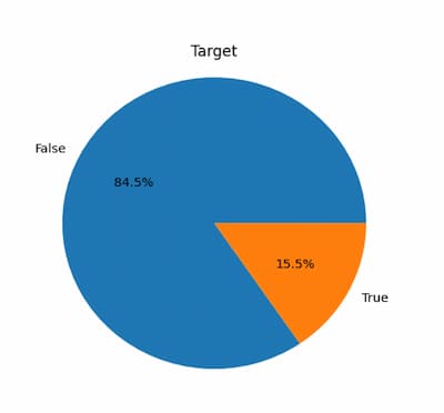
Unbalanced data refers to a situation where the number of instances in one class significantly outweighs the number of instances in the other class. In e-commerce, this could happen if the number of instances in the "buy" class is much smaller than the number of instances in the "not buy" class. The problem with unbalanced data is that classification models trained on such data tend to be biased toward the majority class, leading to poor performance in the minority class.

What is a Classification Model as an ML Algorithm?

A classification model is a machine learning method used to classify or categorize data into distinct classes or groups. A classification model's principal purpose is to uncover patterns in data that may be used to predict the class of new, previously unknown data.

Spam filtering, fraud detection, picture recognition, sentiment analysis, and other applications frequently employ classification models. Classification models are also commonly used in e-commerce to anticipate user behavior, identify prospects, and enhance business performance. A collection of features or characteristics represents the input data in a classification model, and the output is a category variable (i.e., the class label).

Classification models include logistic regression, decision trees, random forests, support vector machines (SVM), and neural networks. Each of these models has advantages and disadvantages and is appropriate for different types of data and activities.

A dataset with labeled examples (data with known class labels) is necessary to train a classification model. After then, the model is trained on this data to understand the patterns that identify the various classes. Once trained, the model may be used to predict the class of fresh, previously unknown data. A classification model's performance is often measured using measures such as accuracy, precision, recall, and F1 score, among others.

Let’s give detailed definitions of these scores to evaluate a classification model:

Accuracy: The proportion of correctly classified samples among all samples. It is a standard evaluation metric for balanced datasets.

Recall: The proportion of true positives (correctly identified minority class samples) among all actual positives (all minority class samples). It is a metric that measures the ability of a model to identify all positive samples.

Precision: The proportion of true positives among all predicted positives. It is a metric that measures the ability of a model to identify positive samples correctly.

F1 score: The harmonic mean of precision and recall. It is a balanced metric that takes into account both false positives and false negatives and is commonly used for imbalanced datasets.

Weighted Avg: An average of precision, recall, and F1 score weighted by the number of samples in each class. It is used to evaluate the overall performance of a model on imbalanced datasets.

Macro avg: An average of precision, recall, and F1 score computed for each class and then averaged. It gives equal weight to each class and evaluates the model’s ability to perform well in all classes.

Precision-Recall Curve: It is a graphical representation that shows the trade-off between the precision and recall of a classification model at different probability thresholds. It is a valuable tool for evaluating the performance of a binary classification model, especially in imbalanced datasets where the distribution of classes is skewed.

Handling Accuracy of Classification Models with Unbalanced Data

One of the biggest challenges for classification models is dealing with unbalanced data, where one class has much more samples than the other. This can lead to skewed forecasts and poor accuracy, which can negatively impact the success of your e-commerce business. Classification models are powerful tools for e-commerce businesses to analyze customer data and make predictions.

There are several methods to handle the accuracy of classification models with unbalanced data in E-commerce. Let's discuss some of them:

1. Resampling Techniques

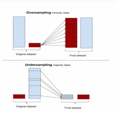
Resampling techniques involve manipulating the data to create a balanced dataset. The two commonly used techniques are undersampling and oversampling. In undersampling, we randomly remove some majority class instances to balance the dataset. In oversampling, we create copies of the minority class instances to balance the dataset. However, oversampling can lead to overfitting, and undersampling can lead to a loss of valuable data.

2. Cost-sensitive Learning

Cost-sensitive learning involves assigning different misclassification costs to different classes. In E-commerce, the cost of misclassifying a "buy" instance as "not buy" could be higher than the cost of misclassifying a "not buy" instance as "buy." By assigning different misclassification costs, the model can focus more on the minority class.

3. Ensemble Methods

Ensemble methods involve combining multiple classification models to improve performance. In E-commerce, we can combine multiple models, each trained on a different subset of the data or using a different algorithm, to create a better-performing model.

4. Using Alternative Performance Metrics

Accuracy is not always the best performance metric to evaluate the performance of a classification model on unbalanced data. Instead, we can use alternative performance metrics such as precision, recall, F1-score, precision-recall curve, or AUC-ROC. These metrics provide a more detailed evaluation of the model's performance on the minority class.

ML engineers utilize these methods and metrics mainly to handle the accuracy of the majority class of output variables in the classification models. However, this technical blog focuses on how one can improve the accuracy of the minority class of the dependent variable as this technical blog describes three powerful techniques you can use to overcome this challenge: Synthetic Minority Oversampling Technique (SMOTE), SHApley Additive exPlanations (SHAP), and Random Forest (RF) model as a case study. By using these techniques, you can improve the accuracy of your classification model and get more reliable results.

Overview of Random Forest Model, SMOTE, and SHAP

Random Forest Model

RF models are a popular machine learning algorithm that is particularly effective for handling unbalanced datasets. RF models work by creating a large number of decision trees and combining their predictions to make a final prediction. By using RF models, we can reduce the bias towards the majority class and improve the accuracy of our classification model.

Random Forest is an ensemble machine learning algorithm that has gained popularity in both classification and regression tasks. It leverages the benefits of multiple decision trees to enhance the accuracy and stability of predictions. Compared to other classification models, Random Forest exhibits several advantages, especially in the context of unbalanced datasets. For instance, it employs a weighted voting scheme to handle the issue of underrepresented minority classes in training data. Moreover, it can manage high-dimensional data with correlated features by randomly selecting a subset of features.

Another significant advantage of Random Forest is that it is not sensitive to class imbalance and can address binary and multi-class problems. Additionally, it exhibits robustness to noisy data, missing values, and irrelevant features. The algorithm offers valuable metrics, such as feature importance scores, that facilitate the identification of the most relevant variables and underlying patterns in the data.

Overall, Random Forest is a versatile tool that can be applied in various domains to improve decision-making and achieve better outcomes.

SMOTE

SMOTE (Synthetic Minority Over-sampling Technique) is a commonly used technique for dealing with unbalanced datasets in machine learning. In an unbalanced dataset, one class may have significantly fewer samples than the other, leading to poor performance of machine learning algorithms that rely on balanced data.

from imblearn.over_sampling import SMOTE
from sklearn.datasets import make_classification
# create an imbalanced dataset
X, y = make_classification(n_classes=2, class_sep=2,
weights=[0.1, 0.9], n_informative=3,
n_redundant=1, flip_y=0, n_features=20,
n_clusters_per_class=1, n_samples=1000,
random_state=10)
# apply SMOTE to balance the dataset
m = SMOTE(random_state=42)
X_res, y_res = sm.fit_resample(X, y)

In this global example, you should first create an unbalanced dataset using scikit-learn's make_classification() function. You then apply the SMOTE algorithm to balance the dataset using the SMOTE() function from the imblearn.over_sampling module. The random_state parameter is set to ensure the reproducibility of the results. Finally, you obtain the balanced dataset by calling the fit_resample() method of the SMOTE object with the original X and y as inputs.

You should notice that after applying SMOTE, the number of instances in the minority class is increased to match the number of instances in the majority class. This may result in a larger dataset overall. The balanced dataset can then be used for training classification models or further analysis.

The SMOTE technique, therefore, generates synthetic samples for the minority class by interpolating between existing samples. The algorithm creates new samples by selecting pairs from the minority class and creating synthetic samples along the line segment that connects them. The number of synthetic samples created is determined by a user-defined parameter. This process continues until the number of samples in the minority class is equivalent to the number of samples in the majority class. By using SMOTE, you can balance the dataset and improve the accuracy of the classification model.

The main advantage of SMOTE is that it helps balance the dataset without additional data collection. This can be especially useful when collecting additional data is expensive or impractical. Moreover, SMOTE has been shown to improve the performance of machine learning models on imbalanced datasets, making it a popular choice for data scientists and machine learning practitioners.

However, it is essential to note that SMOTE is not a universal solution for unbalanced datasets, and its effectiveness may depend on the specific characteristics of the dataset and the machine learning algorithm being used. It is always recommended to experiment with multiple techniques and compare their performance on the dataset of interest before deciding on the best approach.

SHAP

SHAP (SHapley Additive exPlanations) is a model-agnostic method that explains individual predictions in machine learning models, including those used for unbalanced datasets. It is based on the concept of Shapley values from game theory, which is a method for assigning a fair share of the total reward of a cooperative game to each player. In the context of machine learning, SHAP assigns an importance value to each feature for a given prediction, indicating how much each feature contributed to the final result.

For unbalanced datasets, SHAP can be used to understand which features are most important for the majority and minority classes. This can help to identify potential biases in the model and to ensure that the model is not just optimizing for the majority class. Additionally, SHAP can help explain why specific predictions were made, providing insight into the model's decision-making process.

To use SHAP, the first step is to train a machine-learning model on the imbalanced dataset. Once the model is trained, SHAP can be used to calculate the importance value of each feature for a given prediction. By identifying the most critical features for both the majority and minority classes, SHAP can help ensure that the model is not biased and accurately captures all customer segments' behavior.

Here is a general example of Python code:

import shap
from sklearn.ensemble import RandomForestClassifier
# load the dataset
ata = pd.read_csv(“online_shoppers_intention.csv”)
X, y = data.drop(data.target, axis=1), data[‘target’]
X_train, X_test, y_train, y_test = train_test_split(X, y, random_state=0)
# train a Random Forest classifier
clf = RandomForestClassifier(n_estimators=100, random_state=0)
clf.fit(X_train, y_train)
# initialize the SHAP explainer
explainer = shap.TreeExplainer(clf)
# calculate the SHAP values for the testing set
shap_values = explainer.shap_values(X_test)
# plot the SHAP summary plot for the first feature
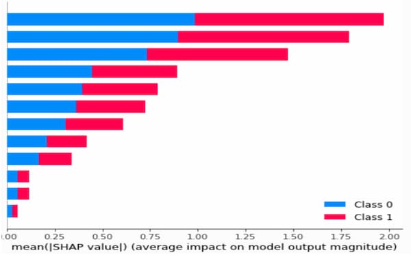
shap.summary_plot(shap_values[0], X_test, feature_names=data.feature_names)

In this code, you see that you first load the dataset and split it into training and testing sets. Then, you train a Random Forest classifier on the training set and initialize a SHAP explainer using the trained model. You should then calculate the SHAP values for the testing set using the shap_values() function and plot a summary plot using the summary_plot() function.

You should notice that the SHAP values are calculated for each feature in the dataset, so the shap_values object is a two-dimensional array. You can plot the SHAP values for each feature using the summary_plot() function, which shows the impact of each feature on the model's output. The feature_names argument is used to label the features in the plot.

SHAP would be the right choice to explain why the RF model makes a particular prediction. This technique is, therefore, helpful in determining which features in the dataset are essential for predicting customer behavior and understanding how the model makes its predictions in the context of e-commerce. SHAP could be used to determine which product features are most important in predicting whether a customer will buy it. Knowing the most significant predictor in forecasting customer behavior can also help e-commerce marketing enhance.

Combining SMOTE and SHAP with RF

Combining SMOTE and SHAP with RF models can improve classification performance on unbalanced data and provide insights into the importance of features for predicting customer behavior.

To combine SMOTE and RF, we first use SMOTE to balance the dataset by generating synthetic instances of the minority class. Then, we train an RF model on the balanced dataset. Finally, we use SHAP to explain the output of the RF model and identify the important features.

Using SMOTE and SHAP with RF models can be computationally intensive, especially for large datasets. However, the insights gained from these techniques can provide valuable information for making informed decisions in E-commerce.

Evaluation of the Performance of the Model on the Minority Class

Evaluating machine learning models' performance is critical to determine their effectiveness and reliability. This is especially important in the case of imbalanced datasets, where the proportion of samples belonging to each class is unequal, and models can easily become biased towards the majority class.

In the upcoming part of the series, we will use an imbalanced dataset; thus, various scoring metrics, including precision, recall, and F1 score, will be employed to evaluate the models' performance. These metrics are commonly used in machine learning to evaluate the quality of binary classification models and provide insight into the model's ability to identify positive and negative samples correctly.

In addition to these metrics, we will also use the macro average, an essential metric for imbalanced datasets. The macro average accounts for the model's performance in both majority and minority classes and provides a more balanced view of the model's overall performance.

To further evaluate the models' performance, we need to plot precision-recall curves and assess the corresponding scores, which are useful criteria for imbalanced datasets. This metric provides a graphical representation of the trade-off between precision and recall, and it can help determine the most suitable threshold for classification.

After modeling, several factors must be considered to ensure the reliability of the obtained scores:

1. Comparing the Train and Test Set Scores

The difference between training and testing data is as follows: training data is used to train the model while testing data is used to verify the model's performance on previously unseen data.

If you achieve good scores on the training set but poor scores on the testing set, you are likely facing an overfitting problem. Overfitting occurs in situations with low bias and high variance, and this means the model has excessively adapted to the training data, effectively memorizing the information rather than learning it.

To handle overfitting, you should utilize techniques such as:

• Increasing the training data
• Reducing model complexity
• Regularization

On the other hand, if you obtain low scores on both the training and testing sets, you are likely facing an underfitting problem. Underfitting occurs in situations with high bias and low variance, which means that the model cannot adapt sufficiently to the training data, resulting in generalization.

To handle underfitting, you should utilize techniques such as:

• Increasing model complexity
• Removing noise from the data
• Increasing training time
• Ensemble methods

2. Cross Validation

Cross-validation is a technique used to evaluate a model's generalization ability. In this process, the dataset is divided into different subsets (folds), and the model is tested on each subset in turn. This helps to measure how well the model can adapt to new and unseen data.

Here's a general example related to Cross Validation:

import numpy as np
from sklearn.ensemble import RandomForestClassifier
from sklearn.model_selection import cross_val_score
from sklearn.pipeline import Pipeline
from sklearn.preprocessing import StandardScaler
data = pd.read_csv(“online_shoppers_intention.csv”)
X, y = data.drop(data.target, axis=1), data[‘target’]
pipeline = Pipeline([
('scaler', StandardScaler()),
('classifier', RandomForestClassifier(random_state=42))
])
cv_scores = cross_val_score(pipeline, X, y, cv=5)
print("Cross-validation scores: ", cv_scores)
print("Mean CV score: ", np.mean(cv_scores))

In the example above, the pipeline created using the Standard Scaler and the Random Forest model is evaluated using 5-fold cross-validation, and the cross-validation scores are computed.

3. GridSearchCV and RandomizedSearchCV

Selecting optimal parameters plays a crucial role in enhancing model performance and determining the best parameters for a given model. Scikit-learn provides two general approaches for this purpose: GridSearchCV, which exhaustively considers all parameter combinations for the specified values, and RandomizedSearchCV, which samples a fixed number of candidates from a parameter space with a defined distribution.

RandomizedSearchCV conducts a random search over the parameters, where each setting is sampled from a distribution of potential parameter values. This method has two primary advantages over a comprehensive search:

• A budget can be determined independently of the number of parameters and their possible values.
• Adding parameters that do not impact performance does not compromise efficiency.

A dictionary is used to specify how parameters should be instantiated, similar to the one for GridSearchCV. Moreover, a computational budget is defined, corresponding to the number of candidates or sampling iterations to be sampled, indicated by the n_iter parameter.

Here's a general example using RandomizedSearchCV:

import numpy as np
from sklearn.ensemble import RandomForestClassifier
from sklearn.model_selection import RandomizedSearchCV
from scipy.stats import randint
data = pd.read_csv(“online_shoppers_intention.csv”)
X, y = data.drop(data.target, axis=1), data[‘target’]
rf_classifier = RandomForestClassifier(random_state=42)
param_dist = {
'n_estimators': randint(10, 200),
'max_depth': randint(1, 10),
'min_samples_split': randint(2, 10),
'min_samples_leaf': randint(1, 10),
}
random_search = RandomizedSearchCV(rf_classifier,
param_distributions=param_dist,
n_iter=50, cv=5, random_state=42)
random_search.fit(X, y)
print("Best parameters: ", random_search.best_params_)
print("Best score: ", random_search.best_score_)

Conclusion

Ultimately, dealing with imbalanced data in e-commerce classification models is super important for making accurate and dependable predictions. This is a big deal in e-commerce since understanding customer behavior and what they like can lead to better marketing strategies and more sales. Using techniques like resampling, cost-sensitive learning, ensemble methods, and different performance metrics, we can make our classification models work better with unbalanced data and be helpful in real-world situations.

It's essential to focus on the minority class's score reliability, especially when working with imbalanced data. Techniques like SMOTE and SHAP can be helpful, but they might have some limitations, so we should be careful when using them. We should always fine-tune the models to ensure they stay reliable and keep up with the ever-changing world of e-commerce.

Also, don't forget about cross-validation and hyperparameter optimization, like GridSearchCV and RandomizedSearchCV. These techniques help our models work better on new, unseen data and improve their overall performance. By being thorough in testing and improving our models, we can create strong classification models that give us valuable insights into customer behavior and help us make better decisions based on data.

In a nutshell, the secret to success in e-commerce classification is knowing the ins and outs of imbalanced data and using the proper techniques to ensure our predictions are accurate and reliable. By constantly experimenting and learning, e-commerce professionals can create and maintain classification models that lead to growth and success in the competitive e-commerce industry.

Upcoming Work

In the next installment of this series, we will address the issue of class imbalance in an e-commerce dataset using various ML algorithms, SMOTE, and SHAP techniques. So, the following text will become a comprehensive applied guideline for handling accuracy issues in unbalanced data. This series will be an important step in understanding customer behavior in the e-commerce industry and will help to develop better marketing strategies.

References

1. https://blog.hubspot.com/service/customer-segmentation?hubs_content=blog.hubspot.com%2Fservice%2Fcustomer-segmentation&hubs_content-cta=What%20is%20customer%20segmentation%3F
2. Chawla, N. V., Bowyer, K. W., Hall, L. O., & Kegelmeyer, W. P. (2002). SMOTE: Synthetic minority over-sampling technique. Journal of artificial intelligence research, 16, 321-357
3. https://machinelearningmastery.com/smote-oversampling-for-imbalanced-classification/
4. https://proceedings.neurips.cc/paper/2017/file/8a20a8621978632d76c43dfd28b67767-Paper.pdf
5. https://bmcbioinformatics.biomedcentral.com/articles/10.1186/1471-2105-10-213
6. https://machinelearningmastery.com/bagging-and-random-forest-for-imbalanced-classification/
7. Chen, Y., Li, H., Liu, S., Liu, J., & Chen, H. (2021). Random Forest for Imbalanced
8. https://towardsdatascience.com/shap-explain-any-machine-learning-model-in-python-24207127cad7
9. https://scikit-learn.org/stable/modules/model_evaluation.html
10. https://en.wikipedia.org/wiki/Overfitting
11. https://www.geeksforgeeks.org/underfitting-and-overfitting-in-machine-learning/
12. https://towardsdatascience.com/overfitting-and-underfitting-principles-ea8964d9c45c
13. https://scikit-learn.org/stable/modules/cross_validation.html
14. https://scikit-learn.org/stable/modules/grid_search.html#grid-search